Using the single template model¶

Quickstart example¶

The single template model is useful for when you know all the intrinsic parameters of your signal (say the masses, spins, etc of a merger). In this case, we don’t need to recalculate the waveform model to sample different possible extrinsic parameters (i.e. distance, sky location, inclination). This can greatly speed up the calculation of the likelihood. To use this model you provide the intrinsic parameters as fixed arguments as in the configuration file below.

This example demonstrates using the single_template model with the dynesty sampler. First, we create the following configuration file:

For this example, we’ll need to download gravitational-wave data for GW170817:

set -e

for ifo in H-H1 L-L1 V-V1
do
    file=${ifo}_LOSC_CLN_4_V1-1187007040-2048.gwf
    test -f ${file} && continue
    curl -O --show-error --silent https://dcc.ligo.org/public/0146/P1700349/001/${file}
done

By setting the model name to single_template we are using SingleTemplate.

Now run:

pycbc_inference \
--config-file `dirname "$0"`/single_simple.ini \
--nprocesses=1 \
--output-file single.hdf \
--seed 0 \
--force \
--verbose

Download

This will run the dynesty sampler. When it is done, you will have a file called single.hdf which contains the results. It should take about a minute or two to run.

To plot the posterior distribution, run:

pycbc_inference_plot_posterior \
--input-file single.hdf \
--output-file single.png \
--z-arg snr

Download

This will create the following plot:

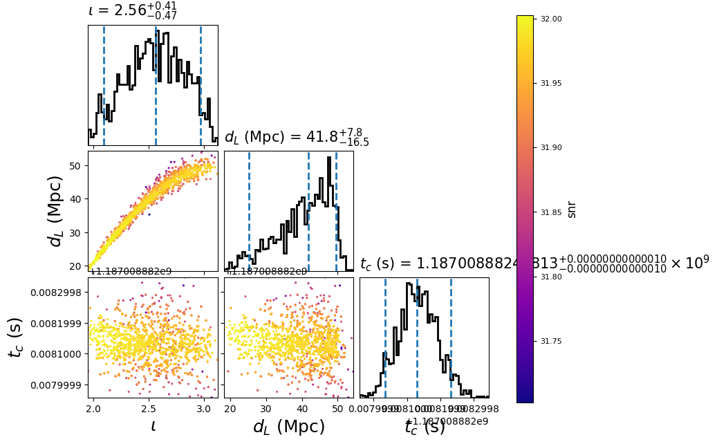
The scatter points show position of different posterior samples. The points are colored by the log likelihood at that point, with the 50th and 90th percentile contours drawn.

Marginalization subset of parameters¶

The single template model supports marginalization over its parameters. This can greatly speed up parameter estimation. The marginalized parameters can also be recovered as in the example below which extends the previous example to include all the parameters the model supports.

In this example, the sampler will only explore inclination, whereas all other parameters are either numerically or analytically marginalized over. Note that the marginalization still takes into account the priors you choose. This includes if you have placed boundaries or constraints.

First, you’ll need the configuration file.

Run this script to use this configuration file:

pycbc_inference \
--config-file `dirname "$0"`/single.ini \
--nprocesses=1 \
--output-file single_marg.hdf \
--seed 0 \
--force \
--verbose

pycbc_inference_plot_posterior \
--input-file single_marg.hdf \
--output-file single_marg.png \
--z-arg snr --vmin 31.85 --vmax 32.15

# This reconstructs any marginalized parameters
# and would be optional if you don't need them or
# have sampled over all parameters directly (see single.ini)
pycbc_inference_model_stats \
--input-file single_marg.hdf \
--output-file single_demarg.hdf \
--nprocesses 1 \
--reconstruct-parameters \
--force \
--verbose

pycbc_inference_plot_posterior \
--input-file single_demarg.hdf \
--output-file single_demarg.png \
--parameters distance inclination polarization coa_phase tc ra dec \
--z-arg snr --vmin 31.85 --vmax 32.15 \

Download

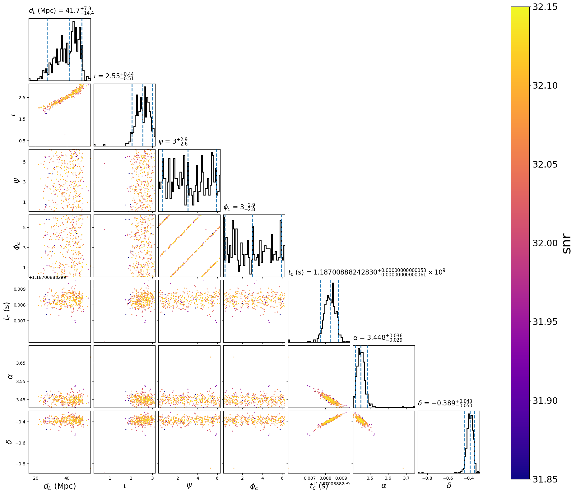
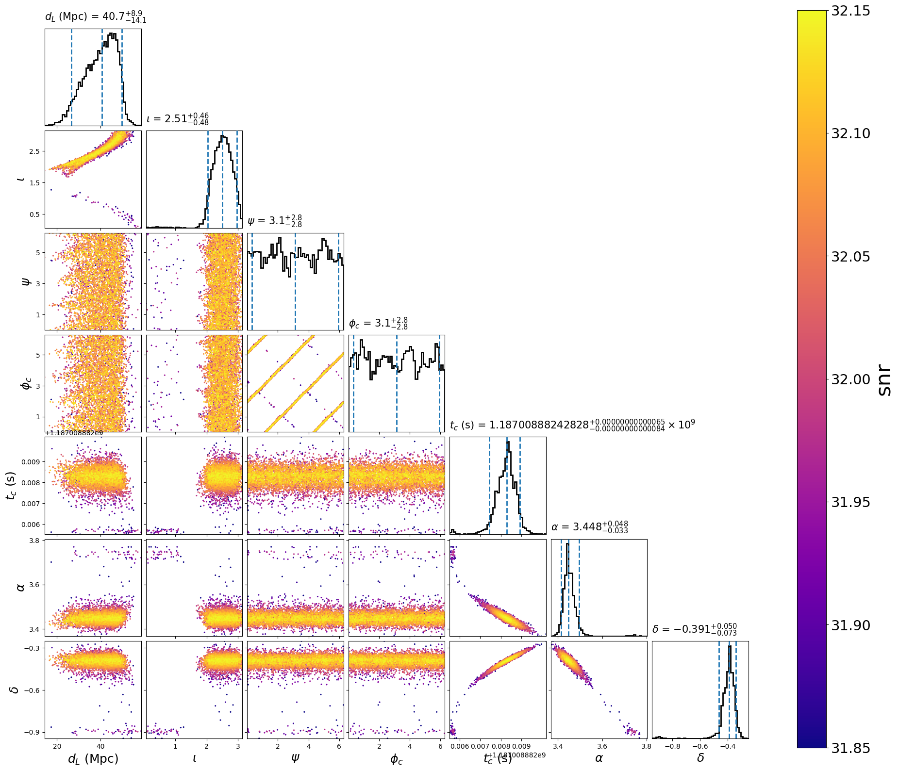
This will create the following plots:

Before demarginalization:

After demarginalization:

Marginalization over all parameters¶

All parameters that the single_template model supports can be marginalized over to do so, you would just configure the model section to include each parameter (minus any you choose to be static). PyCBC Inference will simply reconstruct the missing parameters rather than performing any sampling over the parameter space. The number of samples to take from the posterior is configurable.

First, you’ll need the configuration file. Note that in the sampler section you can set the number of samples to draw from the posterior.

Run this script to use this configuration file:

pycbc_inference \
--config-file `dirname "$0"`/single_instant.ini \
--nprocesses=1 \
--output-file single_instant.hdf \
--seed 0 \
--force \
--verbose

pycbc_inference_plot_posterior \
--input-file single_instant.hdf \
--output-file single_instant.png \
--parameters distance inclination polarization coa_phase tc ra dec \
--z-arg snr --vmin 31.85 --vmax 32.15 \

Download

This will create the following plot:

After demarginalization:

Abitrary sampling coordinates with nested samplers¶

The single template model also supports marginalization over the polarization angle by numerical sampling. The following example features arbitrary sampling coordinates with nested samplers using the fixed_samples distribution. Here we sample in the time delay space rather than sky location directly. This functionality is generic to pycbc inference and could be used with other models or samplers.