Running on an analytic distribution

Several analytic distributions are available to run tests on. These can be run quickly on a laptop to check that a sampler is working properly.

This example demonstrates how to sample a 2D normal distribution with the emcee sampler. First, we create the following configuration file:

[model]
name = test_normal

[sampler]
name = emcee
nwalkers = 5000
niterations = 100

[variable_params]
x =
y =

[prior-x]
name = uniform
min-x = -10
max-x = 10

[prior-y]
name = uniform
min-y = -10
max-y = 10

Download

By setting the model name to test_normal we are using TestNormal. The number of dimensions of the distribution is set by the number of variable_params. The names of the parameters do not matter, just that just that the prior sections use the same names.

Now run:

#!/bin/sh
pycbc_inference --verbose \
        --config-files normal2d.ini \
        --output-file normal2d.hdf \
        --nprocesses 2 \
        --seed 10 \
        --force

Download

This will run the emcee sampler on the 2D analytic normal distribution with 5000 walkers for 100 iterations. When it is done, you will have a file called normal2d.hdf which contains the results. It should take about a minute to run. If you have a computer with more cores, you can increase the parallelization by changing the nprocesses argument.

To plot the posterior distribution after the last iteration, run:

#!/bin/sh
pycbc_inference_plot_posterior --verbose \
        --input-file normal2d.hdf \
        --output-file posterior-normal2d.png \
        --plot-scatter \
        --plot-contours \
        --plot-marginal \
        --z-arg 'loglikelihood:$\log p(h|\vartheta)$' \
        --iteration -1

Download

This will create the following plot:

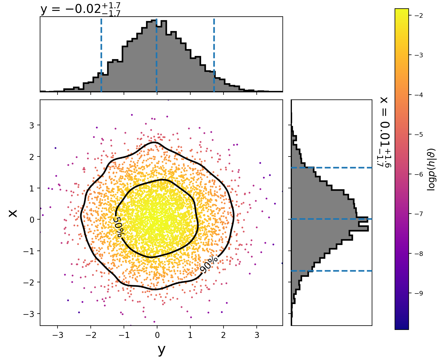
The scatter points show each walker’s position after the last iteration. The points are colored by the log likelihood at that point, with the 50th and 90th percentile contours drawn.

See below for more information about using pycbc_inference_plot_posterior.

To make a movie showing how the walkers evolved, run:

#!/bin/sh
pycbc_inference_plot_movie --verbose \
        --nprocesses 4 \
        --input-file normal2d.hdf \
        --output-prefix frames-normal2d \
        --movie-file normal2d_mcmc_evolution.mp4 \
        --cleanup \
        --plot-scatter \
        --plot-contours \
        --plot-marginal \
        --z-arg 'loglikelihood:$\log p(h|\vartheta)$' \
        --frame-step 1

Download

Note

You need ffmpeg installed for the mp4 to be created.

For more information on pycbc_inference_plot_movie.