Gravitational-wave Detectors

The pycbc.detector module provides the pycbc.detector.Detector class to access information about gravitational wave detectors and key information about how their orientation and position affects their view of a source

Detector Locations

from pycbc.detector import Detector, get_available_detectors

# We can list the available detectors. This gives their detector abbreviation
# along with a longer name. Note that some of these are not physical detectors
# but may be useful for testing or study purposes

for abv in get_available_detectors():
    d = Detector(abv)

    # Note that units are all in radians
    print("{} Latitude {} Longitude {}".format(abv,
                                                  d.latitude,
                                                  d.longitude))

$ python ../examples/detector/loc.py
T1 Latitude 0.6226733602199997 Longitude 2.43536359469
V0 Latitude 0.7615118398400004 Longitude 0.18333805213
V1 Latitude 0.7615118398400004 Longitude 0.18333805213
G1 Latitude 0.9118498275199999 Longitude 0.17116780435
H2 Latitude 0.8107952638300001 Longitude -2.084056769170001
H1 Latitude 0.8107952638300001 Longitude -2.084056769170001
L1 Latitude 0.5334231350600002 Longitude -1.58430937078
I1 Latitude 0.24841853020052615 Longitude 1.3340133249409993
C1 Latitude 0.5963790054099999 Longitude -2.0617574453799996
E1 Latitude 0.7615118398400004 Longitude 0.18333805213
E2 Latitude 0.7629930799000002 Longitude 0.1840585887
E3 Latitude 0.7627046325699999 Longitude 0.1819299673
E0 Latitude 0.7627046325699999 Longitude 0.1819299673
K1 Latitude 0.6355068497000002 Longitude 2.396441015
U1 Latitude 0.0 Longitude 0.0
A1 Latitude 0.53079879206 Longitude -1.5913706849599998
O1 Latitude 0.79156499342 Longitude 0.20853775679
X1 Latitude 0.81070543755 Longitude 0.10821041362
N1 Latitude 0.7299645671 Longitude 0.22117684945999996
B1 Latitude -0.5573418078 Longitude 2.02138216202

Light travel time between detectors

from pycbc.detector import Detector

for ifo1 in ['H1', 'L1', 'V1']:
    for ifo2 in ['H1', 'L1', 'V1']:
        dt = Detector(ifo1).light_travel_time_to_detector(Detector(ifo2))
        print("Direct Time from {} to {} is {} seconds".format(ifo1, ifo2, dt))

$ python ../examples/detector/travel.py
Direct Time from H1 to H1 is 0.0 seconds
Direct Time from H1 to L1 is 0.010012846152267725 seconds
Direct Time from H1 to V1 is 0.027287979933397113 seconds
Direct Time from L1 to H1 is 0.010012846152267725 seconds
Direct Time from L1 to L1 is 0.0 seconds
Direct Time from L1 to V1 is 0.02644834101635671 seconds
Direct Time from V1 to H1 is 0.027287979933397113 seconds
Direct Time from V1 to L1 is 0.02644834101635671 seconds
Direct Time from V1 to V1 is 0.0 seconds

Time source gravitational-wave passes through detector

from pycbc.detector import Detector
from astropy.utils import iers

# Make sure the documentation can be built without an internet connection
iers.conf.auto_download = False

# The source of the gravitational waves
right_ascension = 0.7
declination = -0.5

# Reference location will be the Hanford detector
# see the `time_delay_from_earth_center` method to use use geocentric time
# as the reference
dref = Detector("H1")

# Time in GPS seconds that the GW passes
time = 100000000

# Time that the GW will (or has) passed through the given detector
for ifo in ["H1", "L1", "V1"]:
    d = Detector(ifo)
    dt = d.time_delay_from_detector(dref, right_ascension, declination, time)
    st = "GW passed through {} {} seconds relative to passing by Hanford"
    print(st.format(ifo, dt))

$ python ../examples/detector/delay.py
GW passed through H1 0.0 seconds relative to passing by Hanford
GW passed through L1 0.002444164314882327 seconds relative to passing by Hanford
GW passed through V1 -0.014733669725760679 seconds relative to passing by Hanford

Antenna Patterns and Projecting a Signal into the Detector Frame

from pycbc.detector import Detector
from pycbc.waveform import get_td_waveform

# Time, orientation and location of the source in the sky
ra = 1.7
dec = 1.7
pol = 0.2
inc = 0
time = 1000000000

# We can calcualate the antenna pattern for Hanford at
# the specific sky location
d = Detector("H1")

# We get back the fp and fc antenna pattern weights.
fp, fc = d.antenna_pattern(ra, dec, pol, time)
print("fp={}, fc={}".format(fp, fc))

# These factors allow us to project a signal into what the detector would
# observe

## Generate a waveform
hp, hc = get_td_waveform(approximant="IMRPhenomD", mass1=10, mass2=10,
                         f_lower=30, delta_t=1.0/4096, inclination=inc,
                         distance=400)

## Apply the factors to get the detector frame strain
ht = fp * hp + fc * hc


# The projection process can also take into account the rotation of the
# earth using the project wave function.
hp.start_time = hc.start_time = time
ht2 = d.project_wave(hp, hc, ra, dec, pol)

$ python ../examples/detector/ant.py
No CuPy
No CuPy or GPU PhenomHM module.
No CuPy or GPU response available.
No CuPy or GPU interpolation available.
fp=-0.3854852615415981, fc=0.7059873069668027

Adding a custom detector / overriding existing ones

PyCBC supports observatories with arbitrary locations. For the study of possible new observatories you can add them explicitly within a script or by means of a config file to make the detectors visible to all codes that use the PyCBC detector interfaces.

An example of adding a detector directly within a script.

import matplotlib.pyplot as plt
from pycbc.detector import add_detector_on_earth, Detector
import pycbc.psd
import numpy as np

# Set up potential Cosmic Explorer detector locations

# 40 km detector
lon = -125 / 180.0 * np.pi
lat = 46 / 180.0 * np.pi
yangle = 100.0 / 180.0 * np.pi 
# yangle is the rotation clockwise from pointing north at 0
# xangle can also be specified and allows for detectors that don't have
# 90 degree opening between arms. By default we assume xangle is yangle + pi/2
add_detector_on_earth("C4", lon, lat, yangle=yangle,
                      xlength=40000, ylength=40000)

# 20 km detector
# Arm length is optional, but if provided, you can accurately calcuale
# high-frequency corrects if you provide a frequency argument to the
# antenna pattern method
lon = -94 / 180.0 * np.pi
lat = 29 / 180.0 * np.pi
yangle = 160.0 / 180.0 * np.pi
add_detector_on_earth("C2", lon, lat, yangle=yangle,
                      xlength=20000, ylength=20000)

ra, dec = np.meshgrid(np.arange(0, np.pi*2.0, .1), 
                      np.arange(-np.pi / 2.0, np.pi / 2.0, .1))
ra = ra.flatten()
dec = dec.flatten()

pol = 0
time = 1e10 + 8000 # A time when ra ~ lines up with lat/lon coordinates

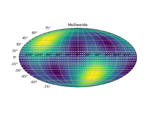
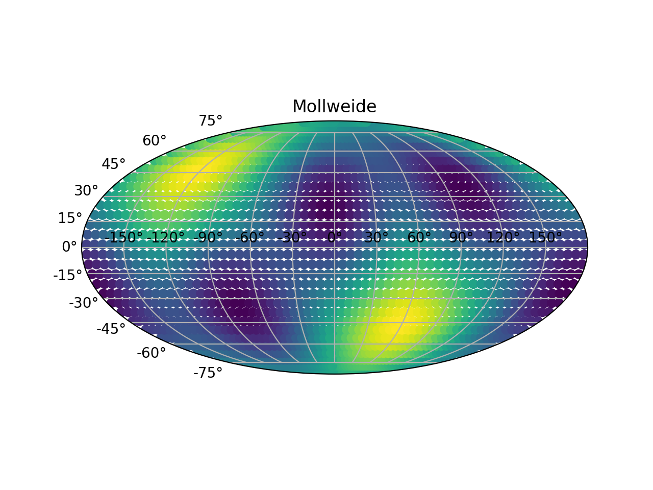
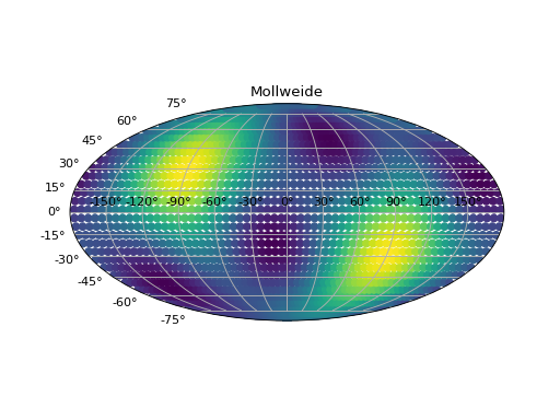
for d in [Detector("C4"), Detector("C2")]:
    fp, fc = d.antenna_pattern(ra, dec, pol, time)

    plt.figure()
    plt.subplot(111, projection="mollweide")
    ra[ra>np.pi] -= np.pi * 2.0
    plt.scatter(ra, dec, c=fp**2.0 + fc**2.0)
    plt.title("Mollweide")
    plt.grid(True)
    plt.show()

(Source code)

_images/custom_00.png — (`png`, `hires.png`, `pdf`)

_images/custom_01.png — (`png`, `hires.png`, `pdf`)

The following demonstrates a config file which similarly can provide custom observatory information. The options are the same as for the direct function calls. To tell PyCBC the location of the config file, set the PYCBC_DETECTOR_CONFIG variable to the location of the file e.g. PYCBC_DETECTOR_CONFIG=/some/path/to/detectors.ini. The following would provide new detectors ‘f1’ and ‘f2’.

[detector-f1]
method = earth_normal
latitude = 0.7120943348136864
longitude = -1.9861846887695471
yangle = 2.0943951023931953

[detector-f2]
method = earth_normal
latitude = -0.5497787143782138
longitude = -2.0594885173533086
yangle = 2.5830872929516078