Filtering
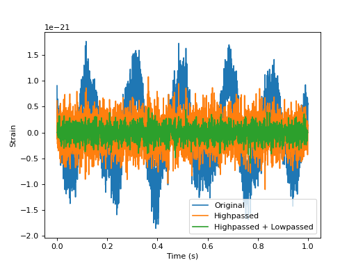
Applying highpass / lowpass filters
import matplotlib.pyplot as pp
import pycbc.noise
import pycbc.psd
import pycbc.filter


# Generate some noise with an advanced ligo psd
flow = 5.0
delta_f = 1.0 / 16
flen = int(2048 / delta_f) + 1
psd = pycbc.psd.aLIGOZeroDetHighPower(flen, delta_f, flow)

# Generate 1 seconds of noise at 4096 Hz
delta_t = 1.0 / 4096
tsamples = int(1 / delta_t)
ts = pycbc.noise.noise_from_psd(tsamples, delta_t, psd, seed=127)
pp.plot(ts.sample_times, ts, label='Original')

# Suppress the low frequencies below 30 Hz
ts = pycbc.filter.highpass(ts, 30.0)
pp.plot(ts.sample_times, ts, label='Highpassed')

# Suppress the high frequencies
ts = pycbc.filter.lowpass_fir(ts, 1000.0, 8)
pp.plot(ts.sample_times, ts, label='Highpassed + Lowpassed')

pp.legend()
pp.ylabel('Strain')
pp.xlabel('Time (s)')
pp.show()
(Source code, png, hires.png, pdf)

Applying an FIR filter
# Apply an FIR filter. The algorithm is written for high performance so if you
# have a large number of taps, it will resort to a FFT based implementation
# under the hood.
import pycbc.types
import pycbc.filter.resample

# Reference time series
ts = pycbc.types.TimeSeries([-1, 1, -1, 1, -1], delta_t=1.0)

# May also be a numpy array
coeff = pycbc.types.Array([1.0, 0, 1.0])

ts_filtered = pycbc.filter.resample.lfilter(coeff, ts)

# If you want to have a zero phase filter provide a symmetric set of coefficients
# The time delay will be compensated for.

ts_filtered2 = pycbc.filter.resample.fir_zero_filter(coeff, ts)
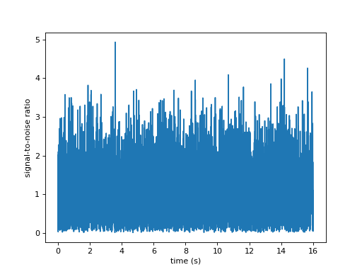
Matched Filter SNR
import matplotlib.pyplot as pp
import pycbc.noise
import pycbc.psd
import pycbc.filter
import pycbc.waveform


# Generate some noise with an advanced ligo psd
flow = 30.0
delta_f = 1.0 / 16
flen = int(2048 / delta_f) + 1
psd = pycbc.psd.aLIGOZeroDetHighPower(flen, delta_f, flow)

# Generate 16 seconds of noise at 4096 Hz
delta_t = 1.0 / 4096
tsamples = int(16 / delta_t)
strain = pycbc.noise.noise_from_psd(tsamples, delta_t, psd, seed=127)
stilde = strain.to_frequencyseries()

# Use a waveform as a matched filter
hp, hc = pycbc.waveform.get_fd_waveform(approximant='IMRPhenomD',
                             mass1=25, mass2=25,
                             f_lower=flow, delta_f=stilde.delta_f)

hp.resize(len(stilde))
snr = pycbc.filter.matched_filter(hp, stilde, psd=psd,
                                      low_frequency_cutoff=flow)


pp.plot(snr.sample_times, abs(snr))
pp.ylabel('signal-to-noise ratio')
pp.xlabel('time (s)')
pp.show()
(Source code, png, hires.png, pdf)

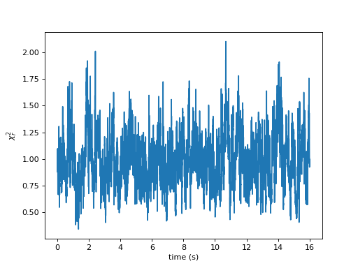
Chisq time series
"""This example shows how to calculate the chi^2 discriminator described in
https://arxiv.org/abs/gr-qc/0405045, also known as the "power chi^2" or "Allen
chi^2" discriminator.
"""

import matplotlib.pyplot as pp
import pycbc.noise
import pycbc.psd
import pycbc.waveform
import pycbc.vetoes


# Generate some noise with an advanced ligo psd
flow = 30.0
delta_f = 1.0 / 16
flen = int(2048 / delta_f) + 1
psd = pycbc.psd.aLIGOZeroDetHighPower(flen, delta_f, flow)

# Generate 16 seconds of noise at 4096 Hz
delta_t = 1.0 / 4096
tsamples = int(16 / delta_t)
strain = pycbc.noise.noise_from_psd(tsamples, delta_t, psd, seed=127)
stilde = strain.to_frequencyseries()

# Calculate the power chisq time series
hp, hc = pycbc.waveform.get_fd_waveform(approximant='IMRPhenomD',
                             mass1=25, mass2=25,
                             f_lower=flow, delta_f=stilde.delta_f)

hp.resize(len(stilde))
num_bins = 16
chisq = pycbc.vetoes.power_chisq(hp, stilde, num_bins, psd,
                                      low_frequency_cutoff=flow)

# convert to a reduced chisq
chisq /= (num_bins * 2) - 2

pp.plot(chisq.sample_times, chisq)
pp.ylabel('$\chi^2_r$')
pp.xlabel('time (s)')
pp.show()
(Source code, png, hires.png, pdf)
