Handling PSDs
Reading / Saving a PSD from a file
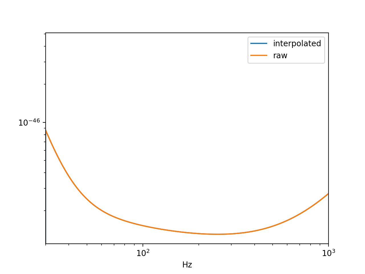
If you have a PSD in a two column, space separated, (frequency strain), you can load this into PyCBC.
import matplotlib.pyplot as pp
import pycbc.psd
import pycbc.types


filename = 'example_psd.txt'

# The PSD will be interpolated to the requested frequency spacing
delta_f = 1.0 / 4
length = int(1024 / delta_f)
low_frequency_cutoff = 30.0
psd = pycbc.psd.from_txt(filename, length, delta_f,
                         low_frequency_cutoff, is_asd_file=False)
pp.loglog(psd.sample_frequencies, psd, label='interpolated')

# The PSD will be read in without modification
psd = pycbc.types.load_frequencyseries('./example_psd.txt')
pp.loglog(psd.sample_frequencies, psd, label='raw')

pp.xlim(xmin=30, xmax=1000)
pp.legend()
pp.xlabel('Hz')
pp.show()

# Save a psd to file, several formats are supported (.txt, .hdf, .npy)
psd.save('tmp_psd.txt')
(Source code, png, hires.png, pdf)
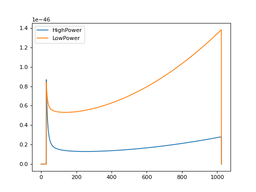
Generating an Analytic PSD from lalsimulation
A certain number of PSDs are built into lalsimulation, which you’ll be able to access through PyCBC. Below we show how to see which ones are available, and demonstrate how to generate one.
import matplotlib.pyplot as pp
import pycbc.psd


# List the available analytic psds
print(pycbc.psd.get_lalsim_psd_list())

delta_f = 1.0 / 4
flen = int(1024 / delta_f)
low_frequency_cutoff = 30.0

# One can either call the psd generator by name
p1 = pycbc.psd.aLIGOZeroDetHighPower(flen, delta_f, low_frequency_cutoff)

# or by using the name as a string.
p2 = pycbc.psd.from_string('aLIGOZeroDetLowPower', flen, delta_f, low_frequency_cutoff)

pp.plot(p1.sample_frequencies, p1, label='HighPower')
pp.plot(p2.sample_frequencies, p2, label='LowPower')
pp.legend()
pp.show()
(Source code, png, hires.png, pdf)
The PSDs from lalsimulation are computed at the required frequencies by interpolating a fixed set of samples; if the required frequencies fall outside of the range of the known samples no warnings will be raised, and (meaningless) extrapolated values will be returned.
Therefore, users should check the validity range of the PSD they are using within lalsimulation, lest they get incorrect results.
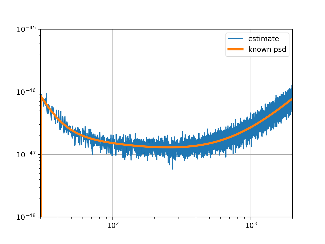
Estimating the PSD of a time series
import matplotlib.pyplot as pp
import pycbc.noise
import pycbc.psd


# generate some colored gaussian noise
flow = 30.0
delta_f = 1.0 / 16
flen = int(2048 / delta_f) + 1
psd = pycbc.psd.aLIGOZeroDetHighPower(flen, delta_f, flow)

### Generate 128 seconds of noise at 4096 Hz
delta_t = 1.0 / 4096
tsamples = int(128 / delta_t)
ts = pycbc.noise.noise_from_psd(tsamples, delta_t, psd, seed=127)

# Estimate the PSD
# We'll choose 4 seconds PSD samples that are overlapped 50 %
seg_len = int(4 / delta_t)
seg_stride = int(seg_len / 2)
estimated_psd = pycbc.psd.welch(ts,
                      seg_len=seg_len,
                      seg_stride=seg_stride)

pp.loglog(estimated_psd.sample_frequencies, estimated_psd, label='estimate')
pp.loglog(psd.sample_frequencies, psd, linewidth=3, label='known psd')
pp.xlim(xmin=flow, xmax=2000)
pp.ylim(1e-48, 1e-45)
pp.legend()
pp.grid()
pp.show()
(Source code, png, hires.png, pdf)
