Signal Processing with GW150914
Here are some interesting examples of how to process LIGO data using GW150914 as an example.
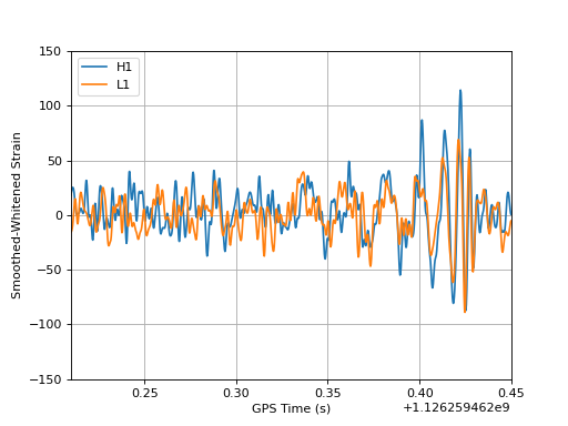
Plotting the whitened strain
import matplotlib.pyplot as pp
from pycbc.filter import highpass_fir, lowpass_fir
from pycbc.psd import welch, interpolate
from pycbc.catalog import Merger


for ifo in ['H1', 'L1']:
    # Read data and remove low frequency content
    h1 = Merger("GW150914").strain(ifo)
    h1 = highpass_fir(h1, 15, 8)

    # Calculate the noise spectrum
    psd = interpolate(welch(h1), 1.0 / h1.duration)

    # whiten
    white_strain = (h1.to_frequencyseries() / psd ** 0.5).to_timeseries()

    # remove some of the high and low
    smooth = highpass_fir(white_strain, 35, 8)
    smooth = lowpass_fir(smooth, 300, 8)

    # time shift and flip L1
    if ifo == 'L1':
        smooth *= -1
        smooth.roll(int(.007 / smooth.delta_t))

    pp.plot(smooth.sample_times, smooth, label=ifo)

pp.legend()
pp.xlim(1126259462.21, 1126259462.45)
pp.ylim(-150, 150)
pp.ylabel('Smoothed-Whitened Strain')
pp.grid()
pp.xlabel('GPS Time (s)')
pp.show()
(Source code, png, hires.png, pdf)
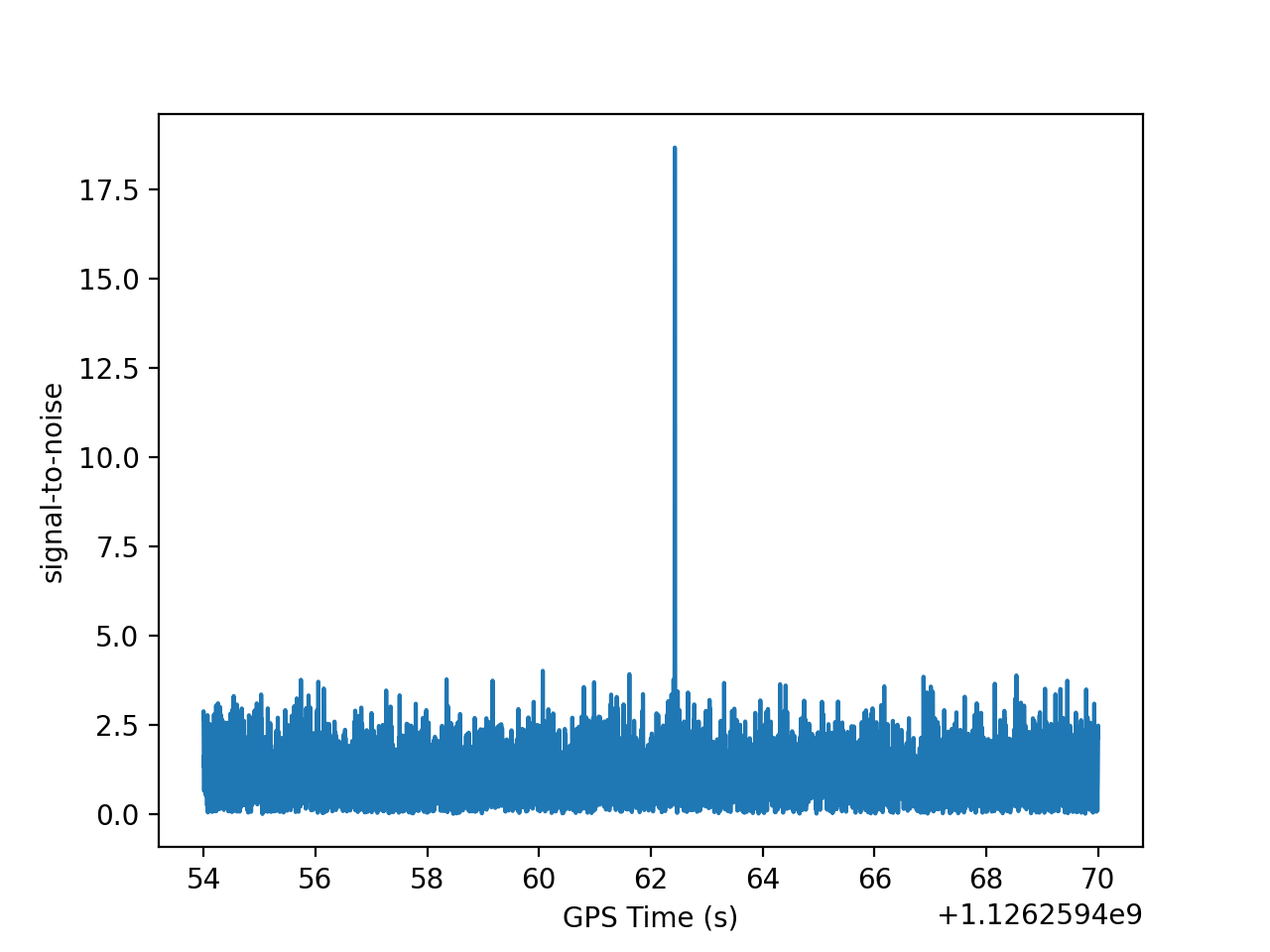
Calculate the signal-to-noise
import matplotlib.pyplot as pp
from urllib.request import urlretrieve
from pycbc.frame import read_frame
from pycbc.filter import highpass_fir, matched_filter
from pycbc.waveform import get_fd_waveform
from pycbc.psd import welch, interpolate


# Read data and remove low frequency content
fname = 'H-H1_LOSC_4_V2-1126259446-32.gwf'
url = "https://www.gwosc.org/GW150914data/" + fname
urlretrieve(url, filename=fname)
h1 = read_frame('H-H1_LOSC_4_V2-1126259446-32.gwf', 'H1:LOSC-STRAIN')
h1 = highpass_fir(h1, 15, 8)

# Calculate the noise spectrum
psd = interpolate(welch(h1), 1.0 / h1.duration)

# Generate a template to filter with
hp, hc = get_fd_waveform(approximant="IMRPhenomD", mass1=40, mass2=32,
                         f_lower=20, delta_f=1.0/h1.duration)
hp.resize(len(h1) // 2 + 1)

# Calculate the complex (two-phase SNR)
snr = matched_filter(hp, h1, psd=psd, low_frequency_cutoff=20.0)

# Remove regions corrupted by filter wraparound
snr = snr[len(snr) // 4: len(snr) * 3 // 4]

pp.plot(snr.sample_times, abs(snr))
pp.ylabel('signal-to-noise')
pp.xlabel('GPS Time (s)')
pp.show()
(Source code, png, hires.png, pdf)

Listen to GW150914 in Hanford
Here we’ll make a frequency shifted and slowed version of GW150914 as it can be heard in the Hanford data.
from pycbc.frame import read_frame
from pycbc.filter import highpass_fir, lowpass_fir
from pycbc.psd import welch, interpolate
from pycbc.types import TimeSeries
try:
    from urllib.request import urlretrieve
except ImportError:  # python < 3
    from urllib import urlretrieve

# Read data and remove low frequency content
fname = 'H-H1_LOSC_4_V2-1126259446-32.gwf'
url = "https://www.gwosc.org/GW150914data/" + fname
urlretrieve(url, filename=fname)
h1 = highpass_fir(read_frame(fname, 'H1:LOSC-STRAIN'), 15.0, 8)

# Calculate the noise spectrum and whiten
psd = interpolate(welch(h1), 1.0 / 32)
white_strain = (h1.to_frequencyseries() / psd ** 0.5 * psd.delta_f).to_timeseries()

# remove some of the high and low frequencies
smooth = highpass_fir(white_strain, 25, 8)
smooth = lowpass_fir(white_strain, 250, 8)

#strech out and shift the frequency upwards to aid human hearing
fdata = smooth.to_frequencyseries()
fdata.roll(int(1200 / fdata.delta_f))
smooth = TimeSeries(fdata.to_timeseries(), delta_t=1.0/1024)

#Take slice around signal
smooth = smooth[len(smooth)//2 - 1500:len(smooth)//2 + 3000]
smooth.save_to_wav('gw150914_h1_chirp.wav')
Note, google chrome may not play wav files correctly, please download to listen.