Waveforms
What waveforms can I generate?
from pycbc.waveform import td_approximants, fd_approximants

# List of td approximants that are available
print(td_approximants())

# List of fd approximants that are currently available
print(fd_approximants())

# Note that these functions only print what is available for your current
# processing context. If a waveform is implemented in CUDA or OpenCL, it will
# only be listed when running under a CUDA or OpenCL Scheme.
$ python ../examples/waveform/what_waveform.py
No CuPy
No CuPy or GPU PhenomHM module.
No CuPy or GPU response available.
No CuPy or GPU interpolation available.
['TaylorT1', 'TaylorT2', 'TaylorT3', 'SpinTaylorT1', 'SpinTaylorT4', 'SpinTaylorT5', 'PhenSpinTaylor', 'PhenSpinTaylorRD', 'EOBNRv2', 'EOBNRv2HM', 'TEOBResum_ROM', 'SEOBNRv1', 'SEOBNRv2', 'SEOBNRv2_opt', 'SEOBNRv3', 'SEOBNRv3_pert', 'SEOBNRv3_opt', 'SEOBNRv3_opt_rk4', 'SEOBNRv4', 'SEOBNRv4_opt', 'SEOBNRv4P', 'SEOBNRv4PHM', 'SEOBNRv2T', 'SEOBNRv4T', 'SEOBNRv4_ROM_NRTidalv2', 'SEOBNRv4_ROM_NRTidalv2_NSBH', 'HGimri', 'IMRPhenomA', 'IMRPhenomB', 'IMRPhenomC', 'IMRPhenomD', 'IMRPhenomD_NRTidalv2', 'IMRPhenomNSBH', 'IMRPhenomHM', 'IMRPhenomPv2', 'IMRPhenomPv2_NRTidal', 'IMRPhenomPv2_NRTidalv2', 'TaylorEt', 'TaylorT4', 'EccentricTD', 'SpinDominatedWf', 'NR_hdf5', 'NRSur7dq2', 'NRSur7dq4', 'SEOBNRv4HM', 'NRHybSur3dq8', 'IMRPhenomXAS', 'IMRPhenomXHM', 'IMRPhenomPv3', 'IMRPhenomPv3HM', 'IMRPhenomXP', 'IMRPhenomXPHM', 'TEOBResumS', 'IMRPhenomT', 'IMRPhenomTHM', 'IMRPhenomTP', 'IMRPhenomTPHM', 'SEOBNRv4HM_PA', 'pSEOBNRv4HM_PA', 'IMRPhenomXAS_NRTidalv2', 'IMRPhenomXP_NRTidalv2', 'IMRPhenomXO4a', 'ExternalPython', 'IMRPhenomXAS_NRTidalv3', 'IMRPhenomXP_NRTidalv3', 'SEOBNRv5_ROM_NRTidalv3', 'IMRPhenomXPNR', 'TaylorF2', 'SEOBNRv1_ROM_EffectiveSpin', 'SEOBNRv1_ROM_DoubleSpin', 'SEOBNRv2_ROM_EffectiveSpin', 'SEOBNRv2_ROM_DoubleSpin', 'EOBNRv2_ROM', 'EOBNRv2HM_ROM', 'SEOBNRv2_ROM_DoubleSpin_HI', 'SEOBNRv4_ROM', 'SEOBNRv4HM_ROM', 'SEOBNRv5_ROM', 'IMRPhenomD_NRTidal', 'SpinTaylorF2', 'TaylorF2NL', 'PreTaylorF2', 'SpinTaylorF2_SWAPPER']
['EccentricFD', 'TaylorF2', 'TaylorF2Ecc', 'TaylorF2NLTides', 'TaylorF2RedSpin', 'TaylorF2RedSpinTidal', 'SpinTaylorF2', 'EOBNRv2_ROM', 'EOBNRv2HM_ROM', 'SEOBNRv1_ROM_EffectiveSpin', 'SEOBNRv1_ROM_DoubleSpin', 'SEOBNRv2_ROM_EffectiveSpin', 'SEOBNRv2_ROM_DoubleSpin', 'SEOBNRv2_ROM_DoubleSpin_HI', 'Lackey_Tidal_2013_SEOBNRv2_ROM', 'SEOBNRv4_ROM', 'SEOBNRv4HM_ROM', 'SEOBNRv4_ROM_NRTidal', 'SEOBNRv4_ROM_NRTidalv2', 'SEOBNRv4_ROM_NRTidalv2_NSBH', 'SEOBNRv4T_surrogate', 'IMRPhenomA', 'IMRPhenomB', 'IMRPhenomC', 'IMRPhenomD', 'IMRPhenomD_NRTidal', 'IMRPhenomD_NRTidalv2', 'IMRPhenomNSBH', 'IMRPhenomHM', 'IMRPhenomP', 'IMRPhenomPv2', 'IMRPhenomPv2_NRTidal', 'IMRPhenomPv2_NRTidalv2', 'SpinTaylorT4Fourier', 'SpinTaylorT5Fourier', 'NRSur4d2s', 'IMRPhenomXAS', 'IMRPhenomXHM', 'IMRPhenomPv3', 'IMRPhenomPv3HM', 'IMRPhenomXP', 'IMRPhenomXPHM', 'SEOBNRv5_ROM', 'IMRPhenomXAS_NRTidalv2', 'IMRPhenomXP_NRTidalv2', 'IMRPhenomXO4a', 'ExternalPython', 'SEOBNRv5HM_ROM', 'IMRPhenomXAS_NRTidalv3', 'IMRPhenomXP_NRTidalv3', 'SEOBNRv5_ROM_NRTidalv3', 'IMRPhenomXPNR', 'SpinTaylorF2_SWAPPER', 'TaylorF2NL', 'PreTaylorF2', 'multiband', 'TaylorF2_INTERP', 'SpinTaylorT5', 'SEOBNRv1_ROM_EffectiveSpin_INTERP', 'SEOBNRv1_ROM_DoubleSpin_INTERP', 'SEOBNRv2_ROM_EffectiveSpin_INTERP', 'SEOBNRv2_ROM_DoubleSpin_INTERP', 'EOBNRv2_ROM_INTERP', 'EOBNRv2HM_ROM_INTERP', 'SEOBNRv2_ROM_DoubleSpin_HI_INTERP', 'SEOBNRv4_ROM_INTERP', 'SEOBNRv4HM_ROM_INTERP', 'SEOBNRv4', 'SEOBNRv4P', 'SEOBNRv5_ROM_INTERP', 'IMRPhenomC_INTERP', 'IMRPhenomD_INTERP', 'IMRPhenomPv2_INTERP', 'IMRPhenomD_NRTidal_INTERP', 'IMRPhenomPv2_NRTidal_INTERP', 'IMRPhenomHM_INTERP', 'IMRPhenomPv3HM_INTERP', 'IMRPhenomXHM_INTERP', 'IMRPhenomXPHM_INTERP', 'SpinTaylorF2_INTERP', 'TaylorF2NL_INTERP', 'PreTaylorF2_INTERP', 'SpinTaylorF2_SWAPPER_INTERP']
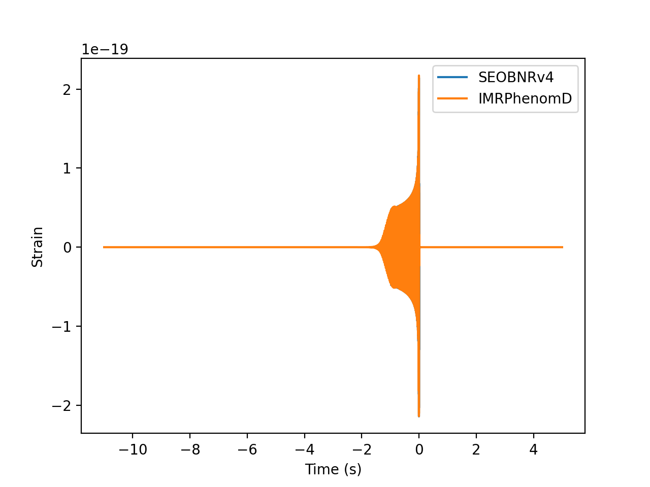
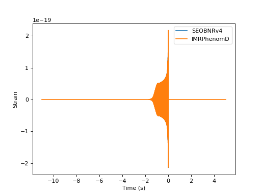
Plotting Time Domain Waveforms
import matplotlib.pyplot as pp
from pycbc.waveform import get_td_waveform


for apx in ['SEOBNRv4', 'IMRPhenomD']:
    hp, hc = get_td_waveform(approximant=apx,
                                 mass1=10,
                                 mass2=10,
                                 spin1z=0.9,
                                 delta_t=1.0/4096,
                                 f_lower=40)

    pp.plot(hp.sample_times, hp, label=apx)

pp.ylabel('Strain')
pp.xlabel('Time (s)')
pp.legend()
pp.show()
(Source code, png, hires.png, pdf)
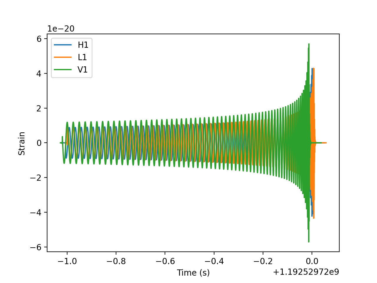
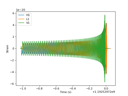
Generating one waveform in multiple detectors
import matplotlib.pyplot as pp
from pycbc.waveform import get_td_waveform
from pycbc.detector import Detector


apx = 'SEOBNRv4'
# NOTE: Inclination runs from 0 to pi, with poles at 0 and pi
#       coa_phase runs from 0 to 2 pi.
hp, hc = get_td_waveform(approximant=apx,
                         mass1=10,
                         mass2=10,
                         spin1z=0.9,
                         spin2z=0.4,
                         inclination=1.23,
                         coa_phase=2.45,
                         delta_t=1.0/4096,
                         f_lower=40)

det_h1 = Detector('H1')
det_l1 = Detector('L1')
det_v1 = Detector('V1')

# Choose a GPS end time, sky location, and polarization phase for the merger
# NOTE: Right ascension and polarization phase runs from 0 to 2pi
#       Declination runs from pi/2. to -pi/2 with the poles at pi/2. and -pi/2.
end_time = 1192529720
declination = 0.65
right_ascension = 4.67
polarization = 2.34
hp.start_time += end_time
hc.start_time += end_time

signal_h1 = det_h1.project_wave(hp, hc,  right_ascension, declination, polarization)
signal_l1 = det_l1.project_wave(hp, hc,  right_ascension, declination, polarization)
signal_v1 = det_v1.project_wave(hp, hc,  right_ascension, declination, polarization)

pp.plot(signal_h1.sample_times, signal_h1, label='H1')
pp.plot(signal_l1.sample_times, signal_l1, label='L1')
pp.plot(signal_v1.sample_times, signal_v1, label='V1')

pp.ylabel('Strain')
pp.xlabel('Time (s)')
pp.legend()
pp.show()
(Source code, png, hires.png, pdf)
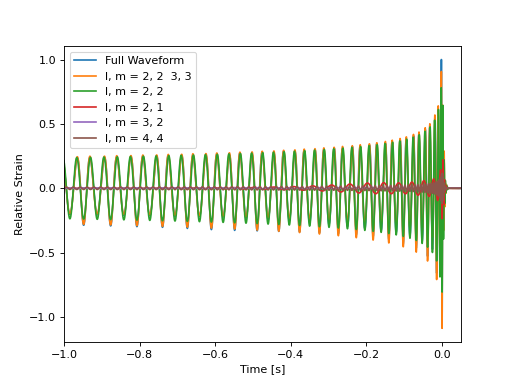
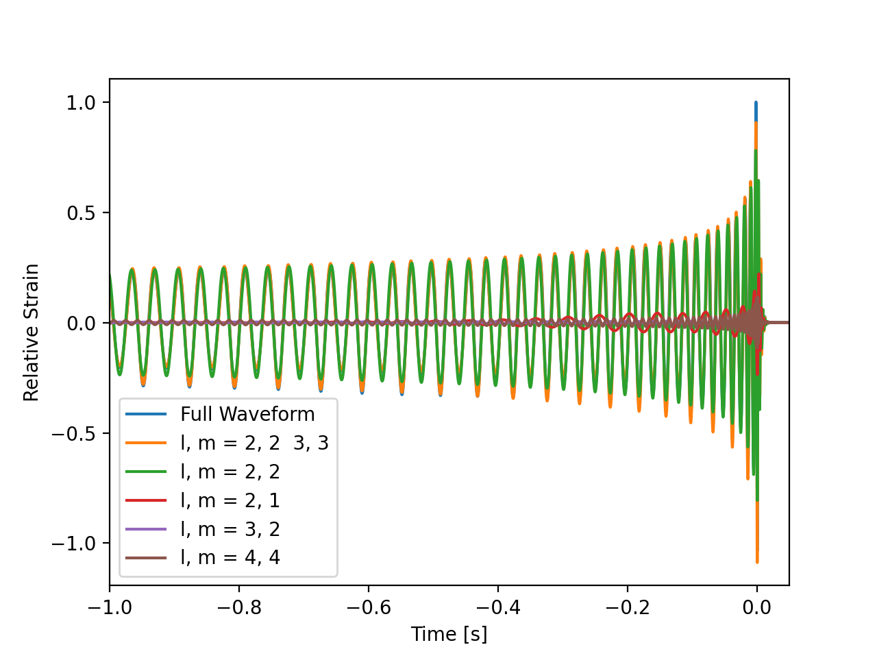
Selecting which modes to include
Gravitational waves can be decomposed into a set of modes. Some approximants only calculate the dominant l=2, m=2 mode, while others included higher-order modes. These often, but not always, include ‘HM’ in the name. The modes present in the output polarizations can be selected for these waveforms as demonstrated below. By default, all modes that the waveform model supports are typically generated.
import matplotlib.pyplot as pp
from pycbc.waveform import get_td_waveform

# Let's plot what our new waveform looks like
pp.figure()

# You can select sets of modes or individual modes using the 'mode_array'
# The standard format is to provide a list of (l, m) modes, however
# a string format is also provided to aid use in population from config files.
# e.g. "22 33" is also acceptable to select these two modes.
# "None" will result in the waveform return its default which is usually
# to return all implemented modes.
for mode_select in [None,
                    [(2, 2), (3, 3)], # Select two modes at once
                    [(2, 2)],
                    [(2, 1)],
                    [(3, 2)],
                    [(4, 4)],
                   ]:
    hp, hc = get_td_waveform(approximant="IMRPhenomXPHM",
                         mass1=7,
                         mass2=40,
                         f_lower=20.0,
                         mode_array=mode_select,
                         inclination = 1.0,
                         delta_t=1.0/4096)


    if mode_select is None:
        label = 'Full Waveform'
        a = hp.max()
    else:
        label = "l, m = " + '  '.join([f"{l}, {m}" for l, m in mode_select])

    (hp / a).plot(label=label)

pp.xlim(-1, 0.05)
pp.legend()
pp.xlabel('Time [s]')
pp.ylabel('Relative Strain')
pp.show()
(Source code, png, hires.png, pdf)

Calculating the match between waveforms
from pycbc.waveform import get_td_waveform
from pycbc.filter import match
from pycbc.psd import aLIGOZeroDetHighPower

f_low = 30
sample_rate = 4096

# Generate the two waveforms to compare
hp, hc = get_td_waveform(approximant="EOBNRv2",
                         mass1=10,
                         mass2=10,
                         f_lower=f_low,
                         delta_t=1.0/sample_rate)

sp, sc = get_td_waveform(approximant="TaylorT4",
                         mass1=10,
                         mass2=10,
                         f_lower=f_low,
                         delta_t=1.0/sample_rate)

# Resize the waveforms to the same length
tlen = max(len(sp), len(hp))
sp.resize(tlen)
hp.resize(tlen)

# Generate the aLIGO ZDHP PSD
delta_f = 1.0 / sp.duration
flen = tlen//2 + 1
psd = aLIGOZeroDetHighPower(flen, delta_f, f_low)

# Note: This takes a while the first time as an FFT plan is generated
# subsequent calls are much faster.
m, i = match(hp, sp, psd=psd, low_frequency_cutoff=f_low)
print('The match is: {:.4f}'.format(m))
$ python ../examples/waveform/match_waveform.py
No CuPy
No CuPy or GPU PhenomHM module.
No CuPy or GPU response available.
No CuPy or GPU interpolation available.
The match is: 0.9534
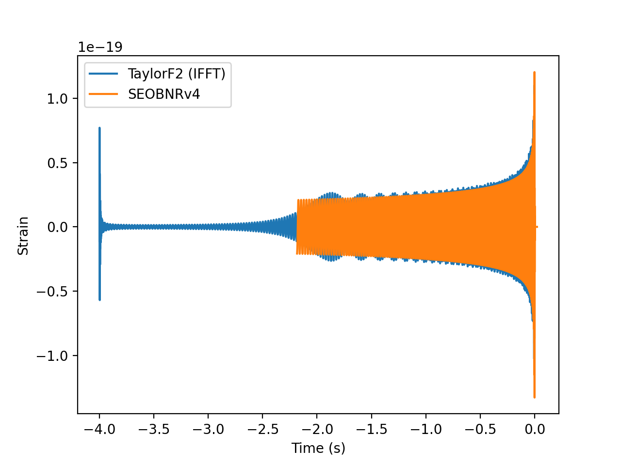
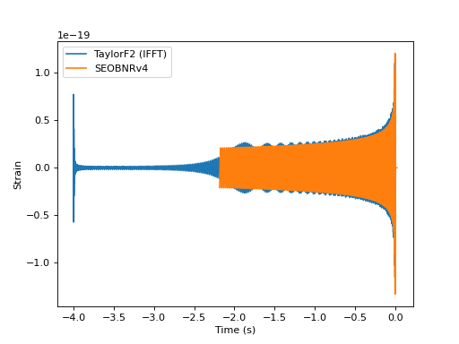
Plotting a TD and FD waveform together in the TD
"""Plot a time domain and Fourier domain waveform together in the time domain.
Note that without special cleanup the Fourier domain waveform will exhibit
the Gibb's phenomenon. (http://en.wikipedia.org/wiki/Gibbs_phenomenon)
"""

import matplotlib.pyplot as pp
from pycbc import types, fft, waveform


# Get a time domain waveform
hp, hc = waveform.get_td_waveform(approximant='SEOBNRv4',
                             mass1=6, mass2=6, delta_t=1.0/4096, f_lower=40)

# Get a frequency domain waveform
sptilde, sctilde = waveform. get_fd_waveform(approximant="TaylorF2",
                             mass1=6, mass2=6, delta_f=1.0/4, f_lower=40)

# FFT it to the time-domain
tlen = int(1.0 / hp.delta_t / sptilde.delta_f)
sptilde.resize(tlen/2 + 1)
sp = types.TimeSeries(types.zeros(tlen), delta_t=hp.delta_t)
fft.ifft(sptilde, sp)

pp.plot(sp.sample_times, sp, label="TaylorF2 (IFFT)")
pp.plot(hp.sample_times, hp, label='SEOBNRv4')

pp.ylabel('Strain')
pp.xlabel('Time (s)')
pp.legend()
pp.show()
(Source code, png, hires.png, pdf)
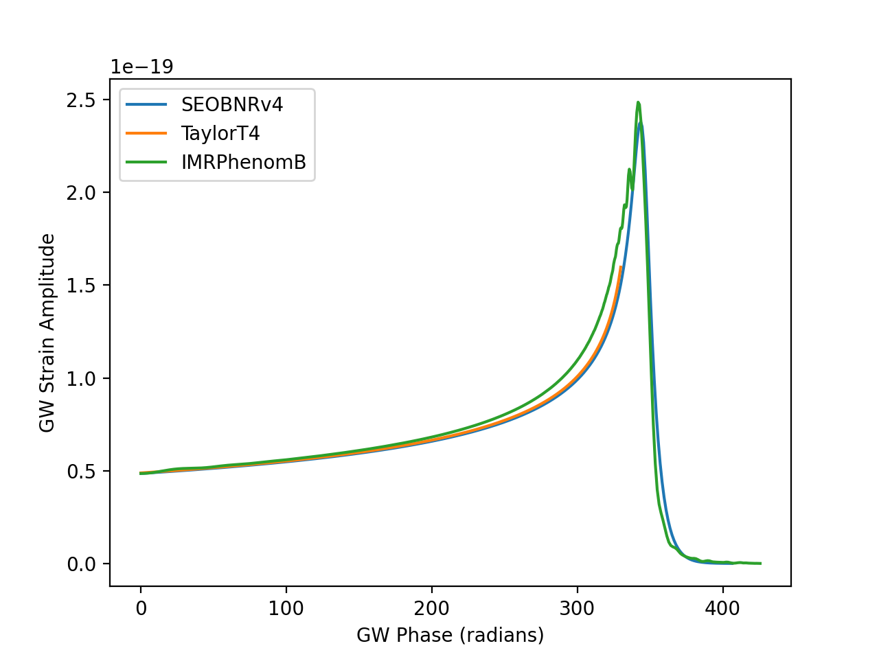
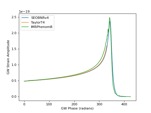
Plotting GW phase and amplitude of TD waveform
import matplotlib.pyplot as pp
from pycbc import waveform


for apx in ['SEOBNRv4', 'TaylorT4', 'IMRPhenomB']:
    hp, hc = waveform.get_td_waveform(approximant=apx,
                                 mass1=10,
                                 mass2=10,
                                 delta_t=1.0/4096,
                                 f_lower=40)

    hp, hc = hp.trim_zeros(), hc.trim_zeros()
    amp = waveform.utils.amplitude_from_polarizations(hp, hc)
    phase = waveform.utils.phase_from_polarizations(hp, hc)

    pp.plot(phase, amp, label=apx)

pp.ylabel('GW Strain Amplitude')
pp.xlabel('GW Phase (radians)')
pp.legend(loc='upper left')
pp.show()
(Source code, png, hires.png, pdf)
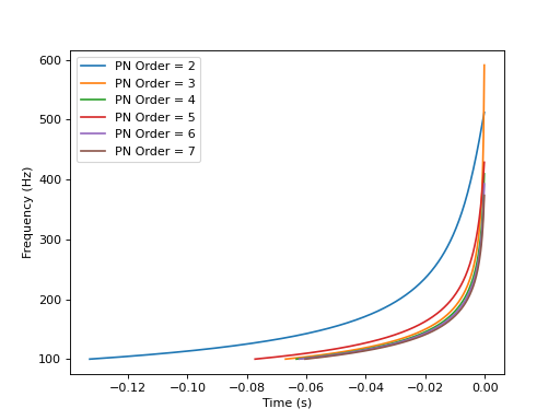
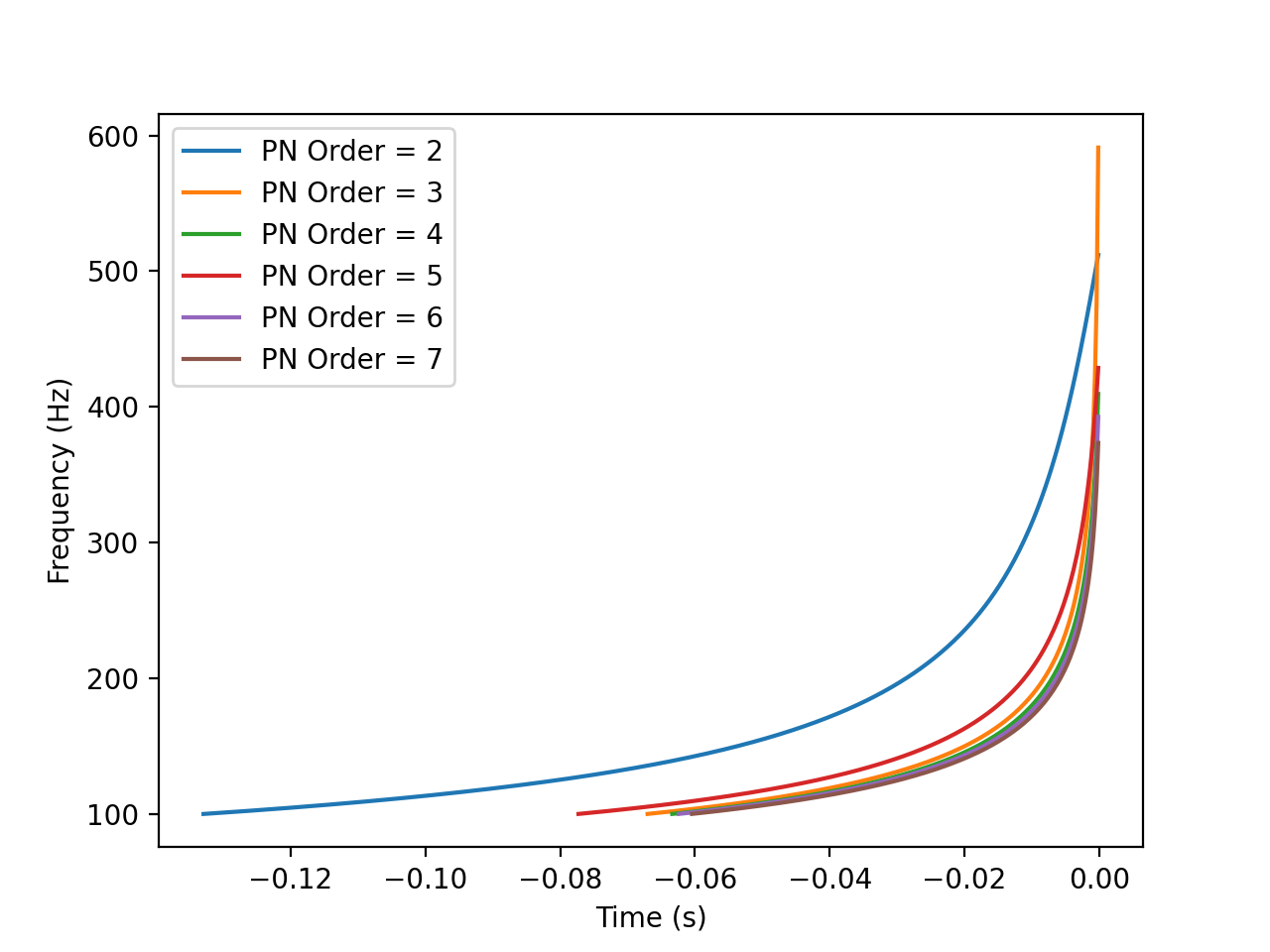
Plotting frequency evolution of TD waveform
import matplotlib.pyplot as pp
from pycbc import waveform


for phase_order in [2, 3, 4, 5, 6, 7]:
    hp, hc = waveform.get_td_waveform(approximant='SpinTaylorT4',
                                 mass1=10, mass2=10,
                                 phase_order=phase_order,
                                 delta_t=1.0/4096,
                                 f_lower=100)

    hp, hc = hp.trim_zeros(), hc.trim_zeros()
    amp = waveform.utils.amplitude_from_polarizations(hp, hc)
    f = waveform.utils.frequency_from_polarizations(hp, hc)

    pp.plot(f.sample_times, f, label="PN Order = %s" % phase_order)

pp.ylabel('Frequency (Hz)')
pp.xlabel('Time (s)')
pp.legend(loc='upper left')
pp.show()
(Source code, png, hires.png, pdf)

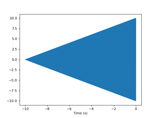
Adding a custom waveform
You can also add your own custom waveform and make it available through the waveform interface standard. You can directly call the code as below or if you include it in a python package, PyCBC can directly detect it!
import numpy
import matplotlib.pyplot as pp
import pycbc.waveform
from pycbc.types import TimeSeries
def test_waveform(**args):
flow = args['f_lower'] # Required parameter
dt = args['delta_t'] # Required parameter
fpeak = args['fpeak'] # A new parameter for my model
t = numpy.arange(0, 10, dt)
f = t/t.max() * (fpeak - flow) + flow
a = t
wf = numpy.exp(2.0j * numpy.pi * f * t) * a
# Return product should be a pycbc time series in this case for
# each GW polarization
#
#
# Note that by convention, the time at 0 is a fiducial reference.
# For CBC waveforms, this would be set to where the merger occurs
offset = - len(t) * dt
wf = TimeSeries(wf, delta_t=dt, epoch=offset)
return wf.real(), wf.imag()
# This tells pycbc about our new waveform so we can call it from standard
# pycbc functions. If this were a frequency-domain model, select 'frequency'
# instead of 'time' to this function call.
pycbc.waveform.add_custom_waveform('test', test_waveform, 'time', force=True)
# Let's plot what our new waveform looks like
hp, hc = pycbc.waveform.get_td_waveform(approximant="test",
f_lower=20, fpeak=50,
delta_t=1.0/4096)
pp.figure(0)
pp.plot(hp.sample_times, hp)
pp.xlabel('Time (s)')
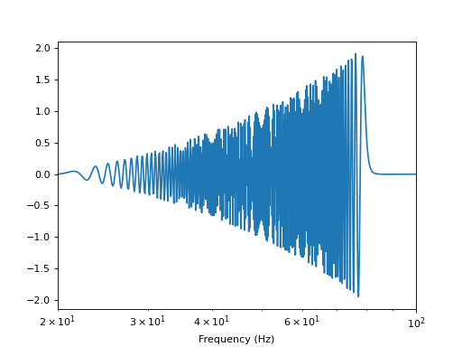
pp.figure(1)
hf = hp.to_frequencyseries()
pp.plot(hf.sample_frequencies, hf.real())
pp.xlabel('Frequency (Hz)')
pp.xscale('log')
pp.xlim(20, 100)
pp.show()
